Algorithm description Iso-Areas
Iso-area from point / Iso-area from layer below. The old advanced “Entry Cost calculation method” parameter has also been removed from every algorithm on this page — entry/exit cost is now always ellipsoidal, using the network layer's own CRS ellipsoid. See Changes from QNEAT3 for the full mapping from QNEAT3.
 Data Source: Stadt Wien – data.wien.gv.at
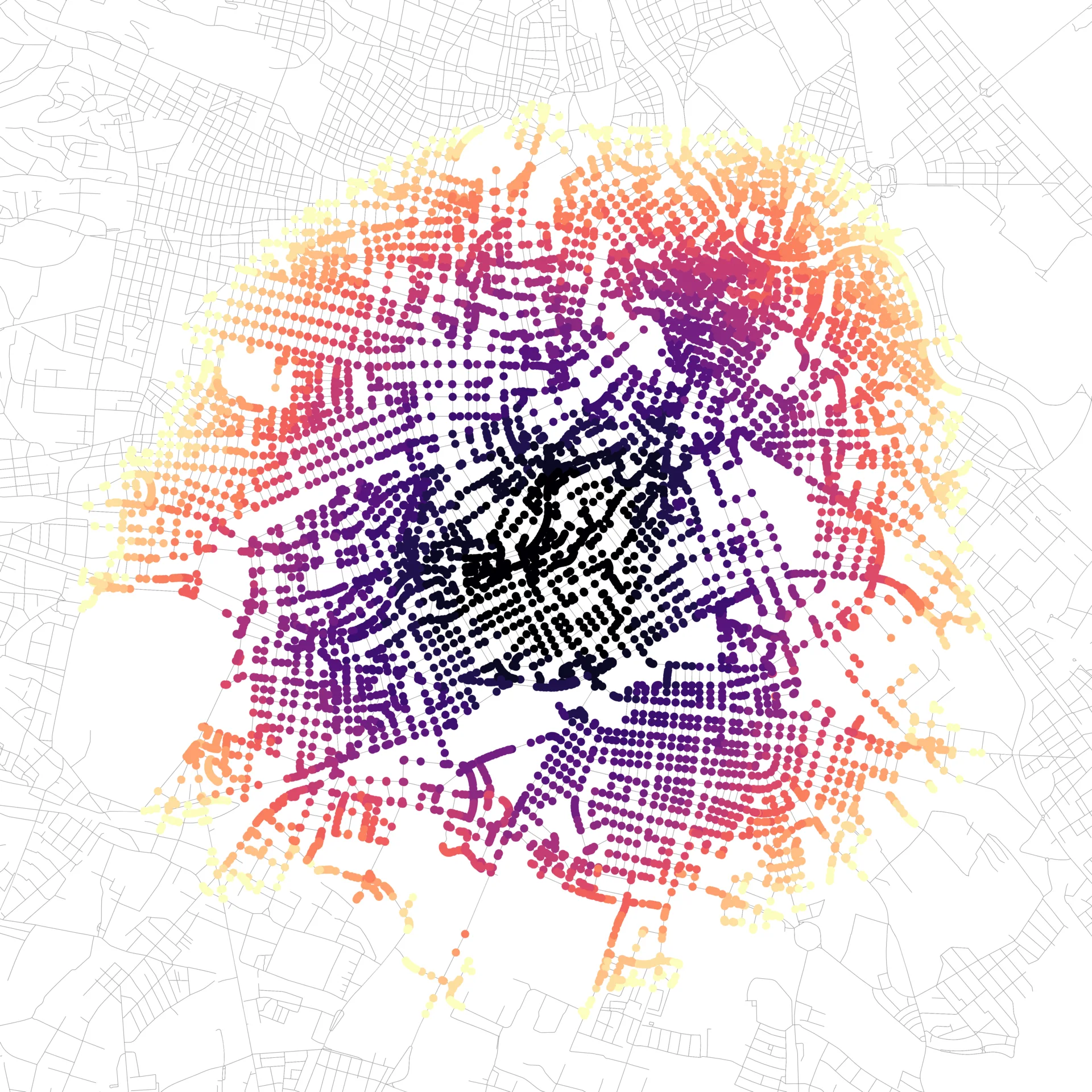
Iso-Area as pointcloud (from point)
This algorithm returns all network nodes reachable within a maximum cost level as a pointcloud, starting from a single manually chosen point. It accounts for points outside of the network (non-network-elements) and increments cost according to distance/default speed. Distances are measured accounting for ellipsoids. You may use the output pointcloud as input for further analyses (eg. nearest-neighbor queries).
| # | Mandatory Parameters | Type | Info |
|---|---|---|---|
| 1 | Network layer | Vector Layer | Geometry type must be LineString |
| 2 | Origin point | Coordinate pair | obtain by clicking on map canvas |
| 3 | Size of iso-area | user input | distance in meters or time in seconds, depending on strategy |
| 4 | Optimization criterion | Shortest | Fastest | - |
| 5 | Output pointcloud | Output Point Layer | Attributes: vertex_id, cost, origin_point_id |
 Data Source: Stadt Wien – data.wien.gv.at
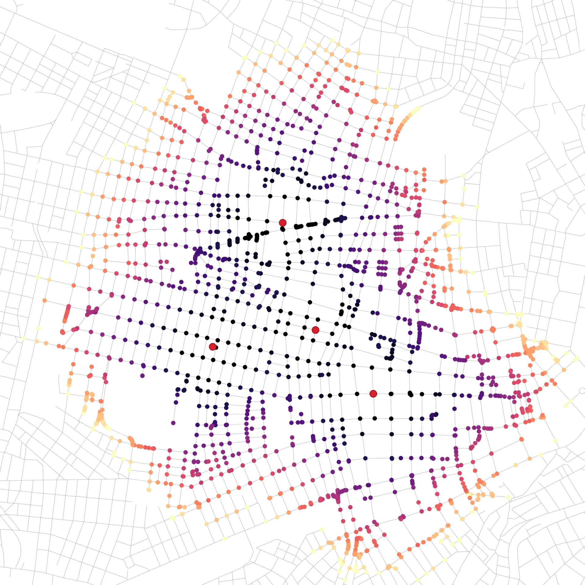
Iso-Area as pointcloud (from layer)
Extends the point-based version above: it queries all network nodes reachable within a maximum cost level starting from every point in a point vector layer, and assigns the nearest origin point's ID to each reachable node.
| # | Mandatory Parameters | Type | Info |
|---|---|---|---|
| 1 | Network layer | Vector Layer | Geometry type must be LineString |
| 2 | Origin point layer | Vector Layer | Geometry must be Point |
| 3 | Unique point ID field | Field | unique identifier for the origin points |
| 4 | Size of iso-area | user input | distance in meters or time in seconds, depending on strategy |
| 5 | Optimization criterion | Shortest | Fastest | - |
| 6 | Output pointcloud | Output Point Layer | Attributes: vertex_id, cost, origin_point_id |
 Data Source: Stadt Wien – data.wien.gv.at
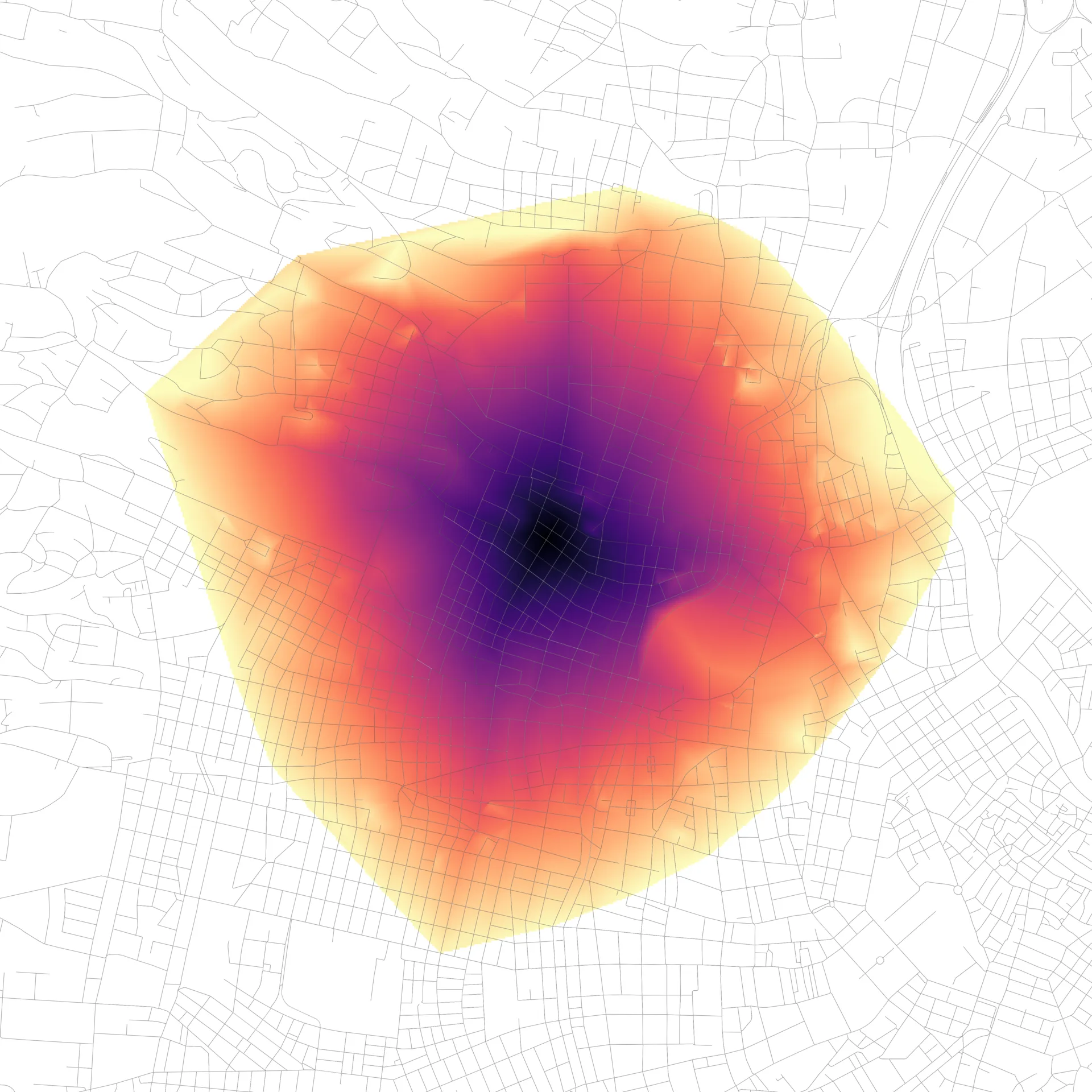
Iso-area as cost surface (from point)
Formerly “Iso-Area as Interpolation (from Point)” — renamed in QNEAT 4.0, see What's New.Note: only use a projected coordinate system (eg. no WGS84) for this kind of analysis.
Returns a network-distance cost surface raster for a maximum cost level, starting from a single manually chosen point. As of 4.0 you can choose the interpolation method: the new Euclidean Distance Transform (fast, works well for dense networks) or the original TIN Interpolation.
| # | Mandatory Parameters | Type | Info |
|---|---|---|---|
| 1 | Network layer | Vector Layer | Geometry type must be LineString |
| 2 | Origin point | Coordinate pair | obtain by clicking on map canvas |
| 3 | Size of iso-area | user input | distance in meters or time in seconds, depending on strategy |
| 4 | Iso-area method | Euclidean Distance Transform | TIN Interpolation | new in 4.0 |
| 5 | Cellsize of interpolation raster | user input | increase default when analyzing larger networks |
| 6 | Optimization criterion | Shortest | Fastest | - |
| 7 | Output cost surface | Output Raster Layer | - |
 Data Source: Stadt Wien – data.wien.gv.at
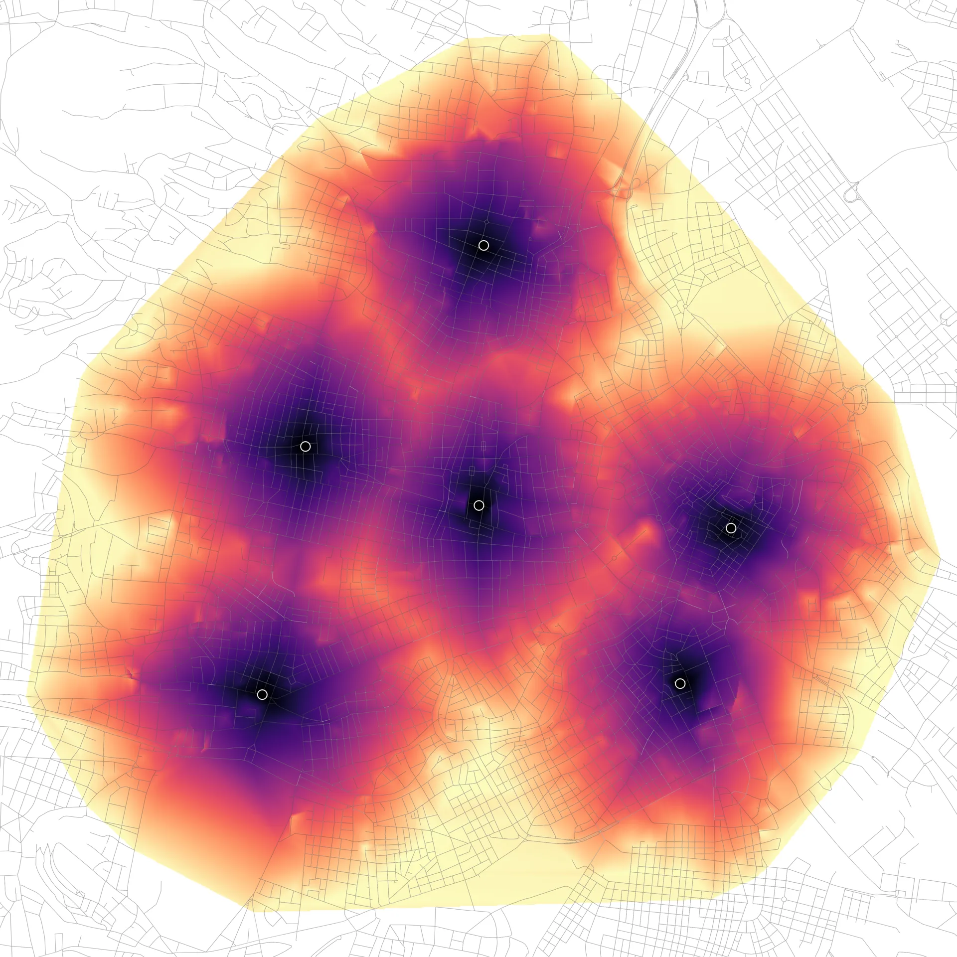
Iso-area as cost surface (from layer)
Formerly “Iso-Area as Interpolation (from Layer)” — renamed in QNEAT 4.0, see What's New.Note: only use a projected coordinate system (eg. no WGS84) for this kind of analysis.
As the point-based algorithm above, but starting from every point in a point vector layer.
| # | Mandatory Parameters | Type | Info |
|---|---|---|---|
| 1 | Network layer | Vector Layer | Geometry type must be LineString |
| 2 | Start points | Vector Layer | Geometry must be Point |
| 3 | Unique point ID field | Field | unique identifier for the start points |
| 4 | Size of iso-area | user input | distance in meters or time in seconds, depending on strategy |
| 5 | Iso-area method | Euclidean Distance Transform | TIN Interpolation | new in 4.0 |
| 6 | Cellsize of interpolation raster | user input | increase default when analyzing larger networks |
| 7 | Optimization criterion | Shortest | Fastest | - |
| 8 | Output cost surface | Output Raster Layer | - |
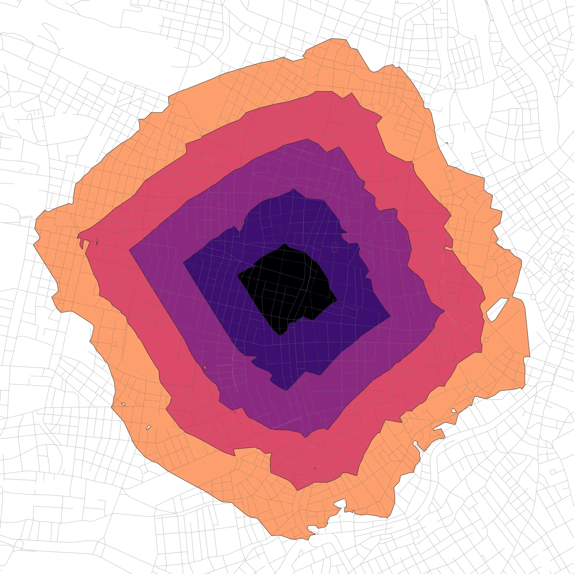
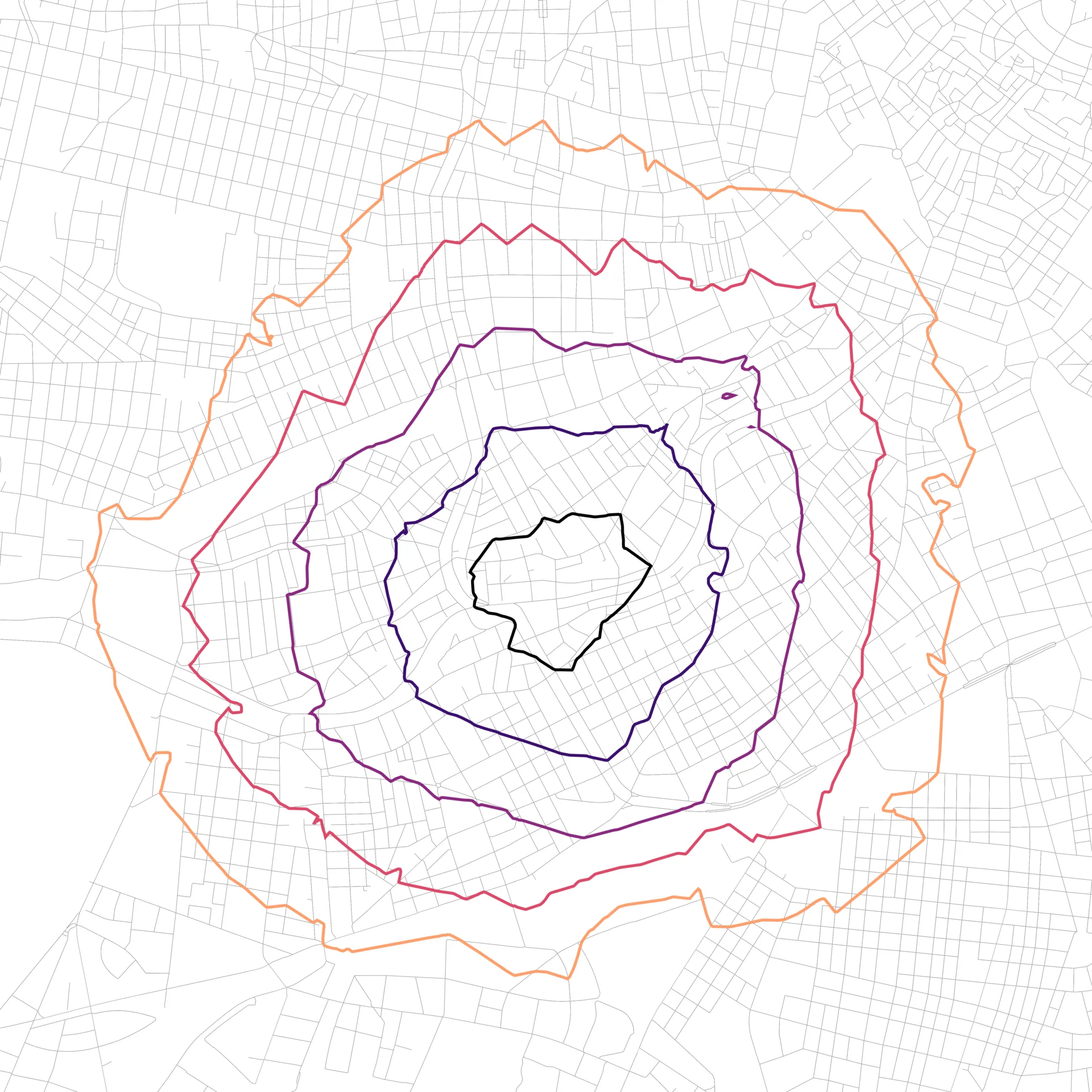
Iso-area from point new in 4.0
Replaces the QNEAT3 matplotlib-based “Iso-Area as Contours (from Point)” and “Iso-Area as Polygons (from Point)” algorithms — see What's New.Note: only use a projected coordinate system (eg. no WGS84) for this kind of analysis.
Returns iso-area polygons or line contours for a maximum cost level and interval, starting from a single manually chosen point. No matplotlib required — polygons/contours are generated with GDAL. Choose the output type (Polygons or Contours) and the underlying method (Euclidean Distance Transform or TIN Interpolation) as parameters.
| # | Mandatory Parameters | Type | Info |
|---|---|---|---|
| 1 | Network layer | Vector Layer | Geometry type must be LineString |
| 2 | Origin point | Coordinate pair | obtain by clicking on map canvas |
| 3 | Iso-area method | Euclidean Distance Transform | TIN Interpolation | - |
| 4 | Iso-area type | Polygons | Contours | - |
| 5 | Size of iso-area | user input | distance in meters or time in seconds, depending on strategy |
| 6 | Contour interval | user input | distance/time value; determines number of bands in the output |
| 7 | Cellsize of interpolation raster | user input | increase default when analyzing larger networks |
| 8 | Optimization criterion | Shortest | Fastest | - |
| 9 | Output cost surface | Output Raster Layer | - |
| 10 | Output iso-areas | Output Vector Layer | Polygons or line contours, depending on iso-area type |
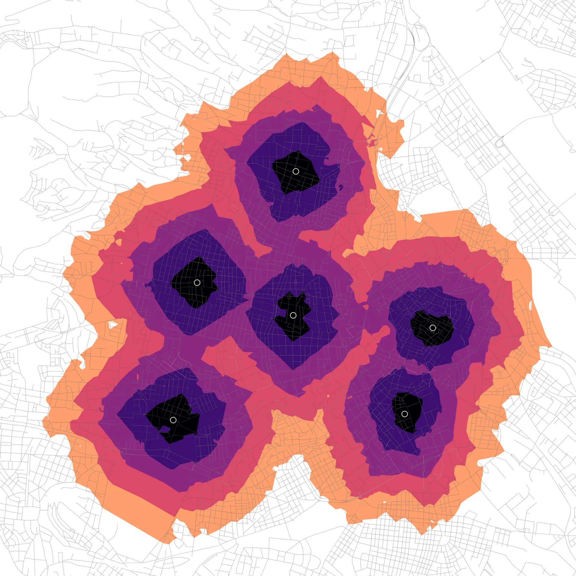
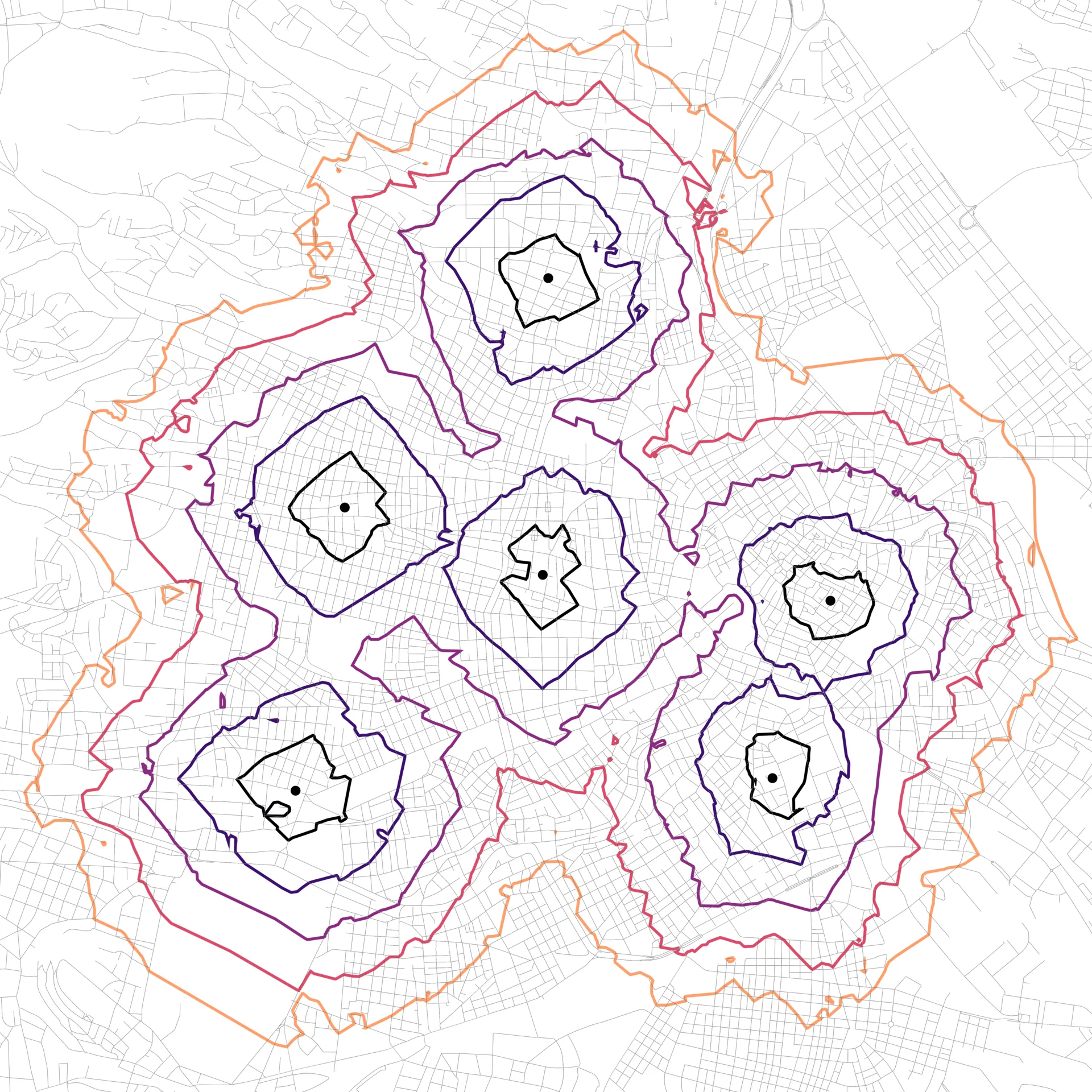
Iso-area from layer new in 4.0
Replaces the QNEAT3 matplotlib-based “Iso-Area as Contours (from Layer)” and “Iso-Area as Polygons (from Layer)” algorithms — see What's New.Note: only use a projected coordinate system (eg. no WGS84) for this kind of analysis.
As the point-based algorithm above, but starting from every point in a point vector layer.
| # | Mandatory Parameters | Type | Info |
|---|---|---|---|
| 1 | Network layer | Vector Layer | Geometry type must be LineString |
| 2 | Origin point layer | Vector Layer | Geometry must be Point |
| 3 | Unique point ID field | Field | unique identifier for the origin points |
| 4 | Iso-area method | Euclidean Distance Transform | TIN Interpolation | - |
| 5 | Iso-area type | Polygons | Contours | - |
| 6 | Size of iso-area | user input | distance in meters or time in seconds, depending on strategy |
| 7 | Contour interval | user input | distance/time value; determines number of bands in the output |
| 8 | Cellsize of interpolation raster | user input | increase default when analyzing larger networks |
| 9 | Optimization criterion | Shortest | Fastest | - |
| 10 | Output cost surface | Output Raster Layer | - |
| 11 | Output iso-areas | Output Vector Layer | Polygons or line contours, depending on iso-area type |
Optional parameters (all Iso-Area algorithms)
The following advanced parameters are shared by every algorithm on this page and implement direction-dependent routing and edge speeds. “Iso-area as cost surface”, “Iso-area from point” and “Iso-area from layer” additionally expose a Maximum off-graph travel cost parameter (Euclidean method only), capping how far a point may be from the network and still be included.
| # | Optional Parameters | Type | Info |
|---|---|---|---|
| 1 | Maximum off-graph travel cost | user input | Euclidean Distance Transform method only; not available on the Pointcloud algorithms |
| 2 | Direction field | Field containing direction values | - |
| 3 | Value for forward direction | user input | input must be referenced to Direction field |
| 4 | Value for backward direction | user input | input must be referenced to Direction field |
| 5 | Value for both directions | user input | input must be referenced to Direction field |
| 6 | Default direction | Forward direction | Backward direction | Both directions | used when no direction field is set, or a feature's direction value doesn't match any of the above |
| 7 | Speed field | Field containing speed values | must be numerical |
| 8 | Default speed (km/h) | user input | (!) sets network entry- and exit-speed |
| 9 | Topology tolerance | user input | Tolerate gaps in network (crs units) |